Modeling horizontal single-axis solar trackers in Energy3D
In the last post, I have blogged about modeling dual-axis solar trackers in Energy3D. To be more precise, the trackers shown in that blog post are altitude-azimuth (Alt/Az), or altazimuth trackers, or AADAT in short. In this post, I will introduce a type of single-axis tracker -- the horizontal single-axis tracker, or HSAT in short.
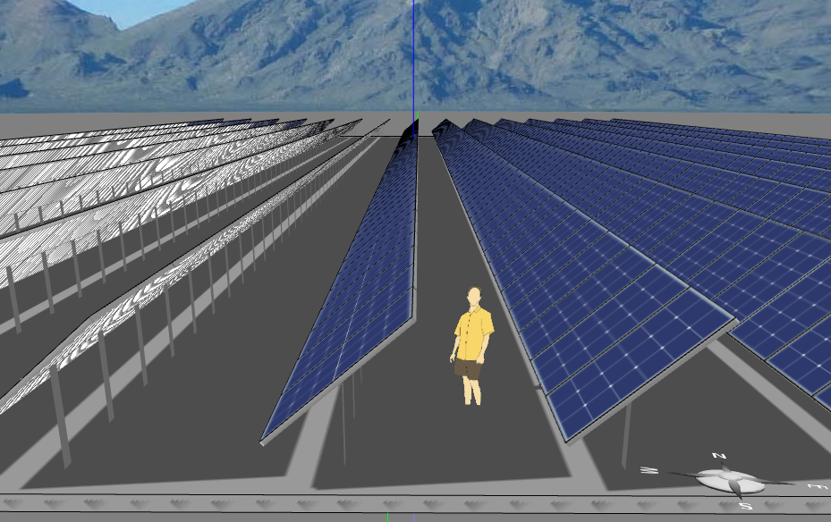
Fig. 1 Solar panel arrays rotated by HSATs
Because single-axis trackers do not need to follow the sun exactly, there are many different designs. Most of them differ in the choice of the axis of rotation. If the axis is horizontal to the ground, the tracker is a HSAT. If the axis is vertical to the ground, the tracker is a vertical single-axis tracker, or VSAT in short. All trackers with axes of rotation between horizontal and vertical are considered tilted single-axis trackers, or TSAT in short. None of these single-axis trackers can help the solar panels capture 100% of the solar radiation that reaches the ground. Exactly which design to choose depends on the location of the solar farm, among other consideration such as the cost of the mechanical system.
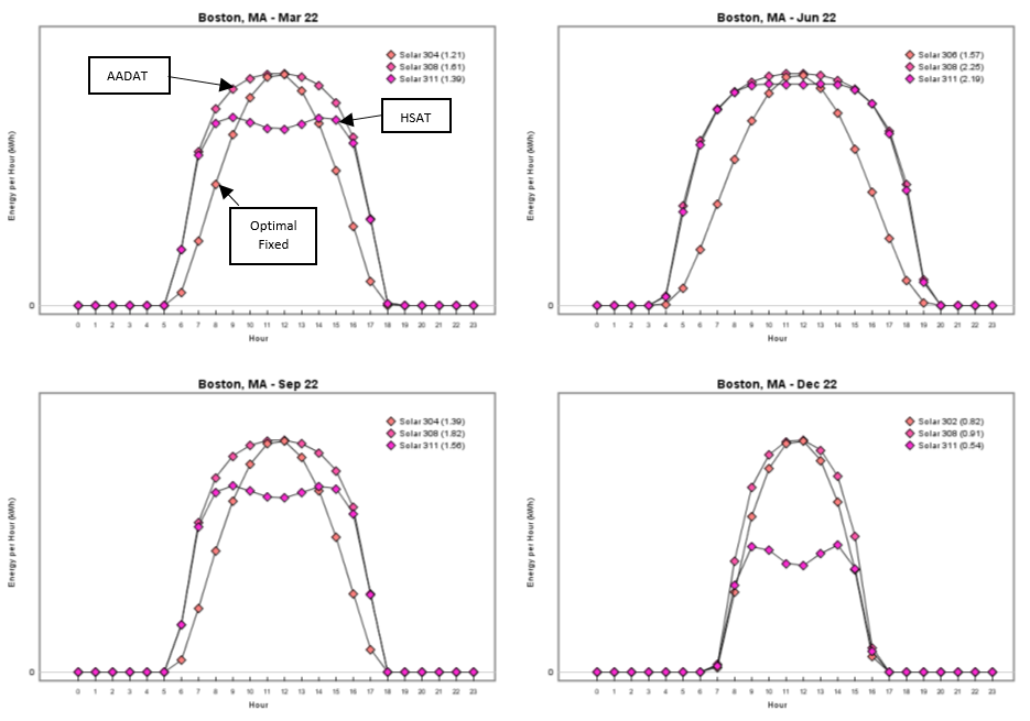
Fig. 2 Compare daily outputs of HSAT, AADAT, and fixed in four seasons.
HSAT is the first type of single-axis tracker that has been implemented in Energy3D. HSAT is probably more common than VSAT and TSAT and is probably easier to construct and install. In most cases, the rotation axis of a HSAT aligns with the north-south direction and the solar panels follow the sun in an east-to-west trajectory, as is shown in the YouTube video embedded in this post and in Figure 1.
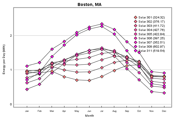
Fig. 3 Compare annual outputs of HSAT, AADAT, and fixed.
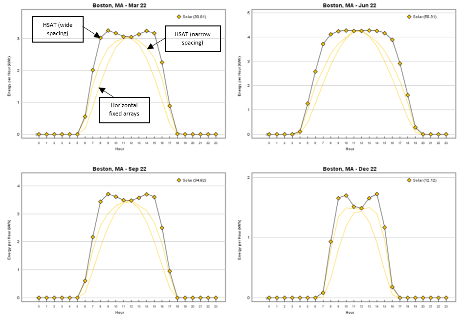
How much more energy can a HSAT help to generate? Figure 2 shows the comparison of the outputs of a HSAT system, an AADAT system, and an optimally fixed solar panel on March 22, June 22, September 22, and December 22, respectively, in the Boston area. The results suggest that the HSAT system is almost as good as the AADAT system in June but its performance declines in March and September and becomes the worst in December (in which case it can only capture a little more than half of the energy harvested by the AADAT system). Interestingly, also notice that there is a dip at noon in the energy graphs for March, September, and December. Why so? I will leave the question for you to figure out. If you have a hard time imagining this, perhaps the visualizations in Energy3D can help.
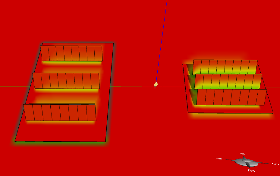
Fig. 4 Compare wide- and narrow-spacing of HSAT arrays
Figure 3 shows the annual result, which suggests that, over the course of a year, the HSAT system -- despite of its relatively unsatisfactory performance in spring, fall, and winter -- still outperforms any fixed solar panel, but it captures about 86% of the energy captured by the AADAT system.
An important factor to consider in solar farm design is the choice of the inter-row spacing to avoid significant energy loss due to shading of adjacent rows in early morning and late afternoon. But you don't want the distance between two rows to be too far as the rows will occupy a large land area that makes no economic sense. With Energy3D, we can easily investigate the change of the energy output with regard to the change of the inter-row spacing. Figure 4 shows the gain from HSAT is greatly reduced when the rows are too close, essentially eliminating the advantages of using solar trackers. Despite of their ability to track the sun, HSATs still require space to achieve the optimal performance.
No comments:
Post a Comment